KV caching

Large language models

Surprisingly, the algorithmic architecture of language models is very simple, but they are computationally inefficient in practice. Modern LLMs follow this rough architecture, with variations and techniques to improve things here and there:

At a high level:

1. Input text is tokenized into subword tokens (e.g. “unhappiness” -> [“un”, “happiness”]).
2. Tokens map to a high-dimensional embedding - an array of a lot of floating point numbers.
3. Transformer blocks process these embeddings, using attention and linear neural network layers to find patterns.
4. The output layer produces a token distribution - a list of how probable every single token is to be the next token.
5. We sample the next token based on the probabilities, add it to the input token sequence, and go back to step 2.

Note that there are a lot of small techniques which are well-used but implied in the diagram. Examples are residual additions, rotary positional embeddings (RoPE), multi-token prediction, causal masking, and so on. For the purposes of this blog post, all you need to know is the high-level idea.

Aside from experimental novel architectures such as diffusion-based language models and state-space models, we’ve mostly been using this architecture since 2017. We still don’t know much about autoregressive transformer-based LLMs in general and have only been gaining incremental improvements since through better training data quality, finding neat prompting or finetuning tricks to fix behavioral patterns, and so on. The biggest reason that they are now so ubiquitous is not likely to be related at all to theoretical and algorithmic advances on the machine learning side, but moreso on the engineering side of things where we’re able to significantly bring down the cost and time required to train and serve better versions of these models. Many of these ideas which come from academia are examples of great engineering, but not many engineers know that such ideas have been pivotal in making LLMs popular.

KV caching

The most popular models are autoregressive. This means that a naive implementation will require you to compute the transformer output of $n$ number of tokens every time you generate the $n$-th token. Without optimizing this, generating a hundred tokens could require thousands of unnecessary attention operations where only a hundred operations would suffice. Consider this naive implementation:

import torch
from transformers import AutoModelForCausalLM, AutoTokenizer

tokenizer = AutoTokenizer.from_pretrained("Qwen/Qwen2.5-0.5B")
model = AutoModelForCausalLM.from_pretrained("Qwen/Qwen2.5-0.5B")
def generate_naive(prompt, max_tokens=128):
    tokens = tokenizer.encode(prompt, return_tensors="pt")

    for _ in range(max_tokens):
        # We perform greedy sampling for implementation simplicity
        logits = model(tokens).logits
        next_token = logits[:, -1, :].argmax()

        # The LLM is allowed to output a token which stops output.
        if next_token.item() == tokenizer.eos_token_id:
            break

        tokens = torch.cat([
            tokens,
            next_token.unsqueeze(0).unsqueeze(0)
        ], dim=-1)

    return tokenizer.decode(tokens[0])

prompt = "Q: What is the capital of France? Explain in 100 words."
completed = generate_naive(prompt)

print(completed)

This code will generate a completion to the prompt, but it’ll also become incrementally slow as it generates more and more tokens. We can see the performance impact of not having a KV cache clearly in this visualization:

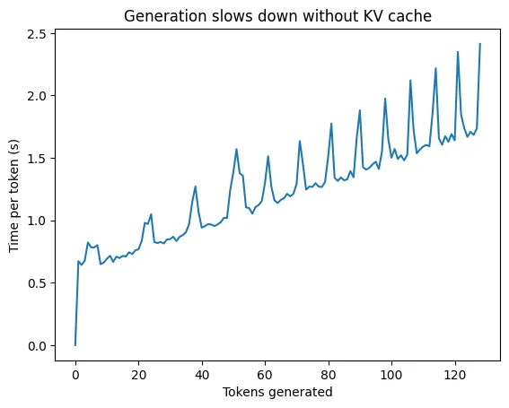
For large prompts, users will notice slowness due to the linear increase in time-per-token. At scale, it’s an infrastructural disaster. With KV caching, we can eliminate a significant amount of computation by caching the intermediary attention values we already computed for previous tokens, resulting in an equally significant improvement in inference times. The key insight is that the attention computations for previous tokens do not change - when we generate token $50$, the attention weights between tokens $10$ and $20$ are exactly the same as they were when we generated token $30$.

import torch
from transformers import AutoModelForCausalLM, AutoTokenizer

tokenizer = AutoTokenizer.from_pretrained("Qwen/Qwen2.5-0.5B")
model = AutoModelForCausalLM.from_pretrained("Qwen/Qwen2.5-0.5B")

def generate_cached(prompt, max_tokens=128):
    tokens = tokenizer.encode(prompt, return_tensors="pt")
    kv_cache = None
    last_token = None
    
    for _ in range(max_tokens):
        # We now save the KV cache on every iteration, saving a lot of time
        if kv_cache is None:
          out = model(tokens, use_cache=True)
        else:
          out = model(last_token, use_cache=True, past_key_values=kv_cache)

        kv_cache = out.past_key_values
        logits = out.logits
        next_token = logits[:, -1, :].argmax()
        last_token = next_token.unsqueeze(0).unsqueeze(0)

        if next_token.item() == tokenizer.eos_token_id:
            break

        tokens = torch.cat([
            tokens,
            next_token.unsqueeze(0).unsqueeze(0),
        ], dim=-1)

    return tokenizer.decode(tokens[0])

prompt = "Q: What is the capital of France? Explain in 100 words."
completed = generate_cached(prompt)

print(completed)

After benchmarking the non-cached and cached variants of the completions function on a nvidia-tesla-t4 on Google Cloud, we can see a clear speedup in inference time:

Inference without KV cache: 159.95s for 128 tokens
Inference with KV cache: 26.60s for 128 tokens
Speedup: 6.012x

Of course, caching the KV of hundreds of tokens during a completion call is expensive in terms of memory, but we’ve also found engineering tricks to get around that as well. There are techniques such as quantization and selective caching, so you’d be hard-pressed to find a production system without any form of caching at all given how much it speeds things up.