The difficult problem of crowd navigation

index

Picture this: you work as a robot operator, and your job is to help the robot safely traverse the length of a busy hallway, littered with humans walking around trying to get places. You have much more important matters to focus on, like playing Solitaire at work, so you want to program it to follow a set of rules so that it can do two things for you automagically:

Maximally reduce the chance of collision with anything - whether it be a person or an object.
While fulfilling goal no. 1, get to its destination as fast as possible.

At first glance, it might seem similar to those pathfinding algorithms that you would generally learn in a computer science curriculum; why not use A* search? If you dabble in reinforcement learning, you might propose using value iteration to let the robot learn an optimal policy through trial and error. If you know a thing or two about deep learning, you might consider using a LSTM or a GAN to map the trajectories of all the agents moving around in the hallway.

The Freezing Robot Problem

Unfortunately, none of the aforementioned algorithms are able to provide an optimal solution to our crowd navigation problem. Many of these methods fail to optimize both objectives - particularly goal no. 2, due to the freezing robot problem. Naive crowd navigation algorithms suffer the problem of causing robots to freeze in place, as they generally fail to find feasible paths in a sufficiently complex crowd.

Yet, for humans that play these navigation games everyday, whether it be in tight sidewalks when walking or intersections when driving, it is generally obvious there is a feasible path in many scenarios where the robot would freeze. For example, if you’re walking dead center on a sidewalk and you see someone going the opposite way in front of you, you don’t keep walking dead center and expect not to collide. In most cases, you and the other person will cooperate by moving either to the left or right, letting each other pass while attempting to avoid coming to a full stop if possible.

A common consensus as to why many algorithms suffer the freezing robot problem is that they implicitly separate the prediction and planning steps of navigating the crowd, preventing the agent’s own planning from negotiating with the environment around it as humans do in real life. To fix this, we need to rethink the problem as a multi-agent equilibrium problem, allowing participants of a crowd to mutually negotiate and cooperatively solve crowd navigation.

A promising angle of study has shown game theory can provide a formal framework for this game of negotiation, allowing us to avoid the a posteriori chicken-and-egg problem of planning using only a costmap model of predicted trajectories - where agents plan after assuming fixed human behaviors. Instead, we begin by reasoning which trajectories are jointly most likely to satisfy both objectives under the assumption that other agents are rational - in the sense that they too will avoid collisions while seeking the fastest route to their destinations. Formally, we are attempting to find the mixed strategy Nash equilibrium (for some utility function $u_i$ encoding individual crowd traversal objectives) such that each agent $p_i$ where $i \in \{1, \cdots, n\}$ follows a mixed strategy

\sigma^{*}_{i} \in \argmax_{\sigma_i \in \Delta(S_i)}\mathop{\mathbb{E}}_{s\sim(\sigma_i, \sigma^{*}_{-i})}[u_i(s)]

Note that agents in real life are not always rational… think of the average driver in America! It’d be cool to see an extension of this work where the components of the individual objective functions for each agent are learned through historical behavioral profiles or data.

Due to the PPAD-completeness of finding a mixed strategy Nash equilibrium, using a generalized algorithm would likely fail to meet the practical realtime constraints of any real-life crowd navigation problem. However, it is known that certain subproblems can be solved with computationally feasible algorithms. As a result, there have been quite a handful of proposed game-theoretic algorithms to optimize crowd traversal. Among these, the Bayesian Recursive Nash Equilibrium algorithm proposed by Sun et al. (2024) stands out by making the problem of finding the global Nash equilibrium tractable for real-time computation at scale.

Bayesian Recursive Nash Equilibrium

The Bayesian Recursive Nash Equilibrium (BRNE) algorithm makes two important observations that allow realtime computability of crowd navigation decisions:

The strategy space $S$ is infinite, so it may be prudent to compute over a sampled subset that represents the strategy space.
While satisfying Nash equilibrium, we want to minimize the system’s overall cost function, which balances collision avoidance and maintaining intent by constraining to the nominal (baseline) strategies $p^{0}$ through a Kullback-Leibler (KL) divergence term:

J(p_1, \cdots, p_N) = \sum^{N}_{i=1}\sum^{N}_{j=i+1}\mathop{\mathbb{E}}_{p_i, p_j}[\text{risk}(s_i, s_j)] + \sum^{N}_{i=1}D(p_i || p^{0}_{i})

To represent strategies, each agent is initialized with a sampled subset of trajectories from a uniform nominal Gaussian process conditioned by a trajectory produced by a high-level meta-planner. In the simple scenario where we have no static obstacles, we condition the nominal Gaussian process such that its mean goes from the agent’s current position to the goal position. To begin sampling trajectories, we first find the Cholesky decomposition of the nominal Gaussian process.

import numpy as np
import matplotlib.pyplot as plt
from sklearn.gaussian_process.kernels import RBF, ConstantKernel

dt = 0.3
tsteps = 20
num_samples = 200

# Initial positions of the agents
init_1, goal_1 = np.array([0.0, 1.0]), np.array([6.0, -1.0])
init_2, goal_2 = np.array([6.0, 1.0]), np.array([0.0, -1.0])

kernel = ConstantKernel(5.0) * RBF(length_scale=np.sqrt(1 / (2 * 0.03)))

# Compute the Cholesky decomposition for the Gaussian process
t_cond = np.array([0.0, (tsteps - 1) * dt]).reshape(-1, 1)
t_all = (np.arange(tsteps) * dt).reshape(-1, 1)

mat_11 = kernel(t_cond, t_cond)
mat_12 = kernel(t_cond, t_all)
mat_22 = kernel(t_all, t_all)

cov = mat_22 - mat_12.T @ np.linalg.inv(mat_11) @ mat_12
cov = cov + (np.eye(tsteps) * 1e-4)

cholesky = np.linalg.cholesky(cov)

We then generate Gaussian process samples using the Cholesky decomposition:

def generate_gp_samples(init, goal, lcov):
    mean = np.linspace(init, goal, tsteps)
    samples = []

    for _ in range(num_samples):
        z_x = np.random.randn(tsteps)
        sample_x = lcov @ z_x + mean[:, 0]
        
        z_y = np.random.randn(tsteps)
        sample_y = lcov @ z_y + mean[:, 1]
        
        traj = np.stack([sample_x, sample_y], axis=1)
        samples.append(traj)

    return np.array(samples)

samples_1 = generate_gp_samples(init_1, goal_1, cholesky)
samples_2 = generate_gp_samples(init_2, goal_2, cholesky)

To see what we just did, let’s graph the samples we generated from the code snippet above:

def plot(samples_1=None, samples_2=None, weights_1=None, weights_2=None, opt_1=None, opt_2=None):
    fig, ax = plt.subplots(figsize=(6, 6))
    
    if samples_1 is not None:
        w1 = weights_1 or np.ones(len(samples_1))
        w2 = weights_2 or np.ones(len(samples_2))
        
        for i, s in enumerate(samples_1):
            ax.plot(s[:, 0], s[:, 1], "C0", alpha=0.1 * w1[i], linewidth=2)
        for i, s in enumerate(samples_2):
            ax.plot(s[:, 0], s[:, 1], "C1", alpha=0.1 * w2[i], linewidth=2)
    
    if opt_1 is not None:
        ax.plot(opt_1[:, 0], opt_1[:, 1], "C0", linewidth=3)
    if opt_2 is not None:
        ax.plot(opt_2[:, 0], opt_2[:, 1], "C1", linewidth=3)
    
    ax.plot(*init_1, "oC0", ms=12, label="Agent 1")
    ax.plot(*goal_1, "sC0", ms=12)
    ax.plot(*init_2, "oC1", ms=12, label="Agent 2")
    ax.plot(*goal_2, "sC1", ms=12)
    ax.axis("equal")
    ax.axis("off")
    ax.legend()

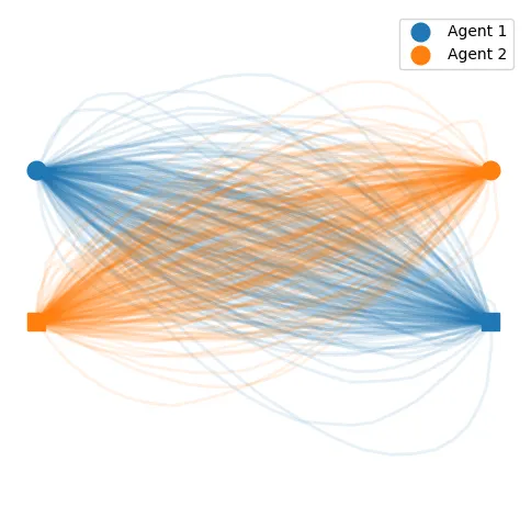
plot(samples_1, samples_2)

Initially, the samples should show the nominal uniform distribution of trajectories:

A picture of the nominal trajectory samples

In order to find equilibria, we must optimize this initially uniform distribution by weighing the varying samples based on the individual objective function $J_i(p_1, \cdots, p_n)$ . The first order of business is to define the collision risk function used to maximize the agent collision avoidance behavior. As the risk function is arbitrary, we implement the one used by the authors of the BRNE paper.

risk_cov = np.diag(np.random.uniform(low=0.3, high=0.8, size=2)) * 0.5
risk_cov[0, 1] = np.sqrt(np.prod(np.diagonal(risk_cov))) / 2.0
risk_cov[1, 0] = risk_cov[0, 1]
risk_cov_inv = np.linalg.inv(risk_cov)

def risk(traj_1, traj_2):
    d_traj = traj_1 - traj_2
    vals = np.exp(-0.5 * np.sum(d_traj @ risk_cov_inv * d_traj, axis=1)) * 200.0
    return np.mean(vals)

Once the aforementioned components are implemented, it is possible to run BRNE to find Nash equilibria. The goal is to run the algorithm continuously for an agent - such as a robot - to make decisions in real-time. In fact, the BRNE paper claims that they are able to compute an entire BRNE planning cycle in $3.9 \pm 0.1$ ms for a two-agent game on a laptop with an Intel i9-12900K with 20 threads using Numba. Let’s implement the planning iteration loop as shown below:

num_iters = 20
weights_1 = np.ones(num_samples)
weights_2 = np.ones(num_samples)

risk_table = np.zeros((num_samples, num_samples))
for i in range(num_samples):
    for j in range(num_samples):
        risk_table[i, j] = risk(samples_1[i], samples_2[j])

for _ in range(num_iters):
    risk_2to1 = np.mean(risk_table * weights_2, axis=1)
    new_weights_1 = np.exp(-1.0 * risk_2to1)
    new_weights_1 /= np.mean(new_weights_1)
    
    risk_1to2 = np.mean(risk_table * new_weights_1[:, None], axis=0)
    new_weights_2 = np.exp(-1.0 * risk_1to2)
    new_weights_2 /= np.mean(new_weights_2)
    
    weights_1 = new_weights_1
    weights_2 = new_weights_2

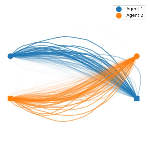
plot(samples_1, samples_2, weights_1, weights_2)

Once we plot the samples weighted by the learned strategy probabilities of each trajectory, we find a much less uniform visualization of the previously nominal strategy:

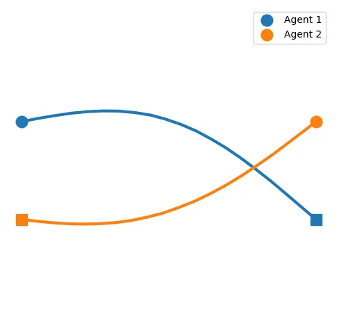
A picture of the optimized trajectory samples

We can compute the best mixed strategy for the agent by taking these weighted trajectories and averaging them into a single trajectory:

opt_traj_1 = np.mean(samples_1 * weights_1[:, None, None], axis=0)
opt_traj_2 = np.mean(samples_2 * weights_2[:, None, None], axis=0)

plot(samples_1, samples_2, opt_1=opt_traj_1, opt_2=opt_traj_2)

A picture of the optimized mean paths

And you’re done! After you complete the trivial (not really) task of digitalizing the hallway environment and its agents, your robot will run this algorithm hundreds of times every second and leave in you in peace to play Solitaire.

KV caching

The difficult problem of crowd navigation

The Freezing Robot Problem

Game-Theoretic Crowd Navigation

Bayesian Recursive Nash Equilibrium